
Right. Time to close the UCL chapter.
The actual project finished before the blog did. I am choosing to describe this as an unusually thorough editorial process.
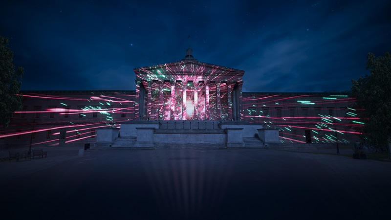
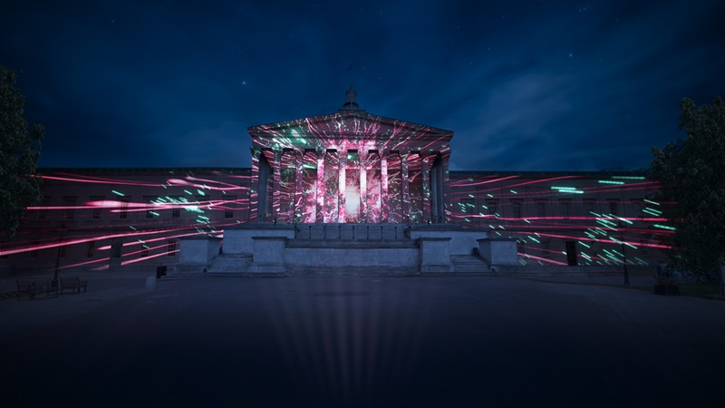
Figure 1. Artist’s impression of UCL Illuminated, showing the Portico and Wilkins Building lit up for UCL’s bicentenary celebrations in 2026. Image credit: © Double Take Productions. Source: UCL News.
Over the previous posts, I’ve covered simulated collisions, boosted Higgs tagging, disagreements between model implementations, and the eventual adventure into Contur and Spey.
So, what did I actually achieve? And if I returned to the project, where would I start?
The original question
My BSc project, supervised by Professor Jon Butterworth, investigated Higgs physics at the Future Circular Collider, focusing on associated ZH production at 85 TeV.
The signature was an invisibly decaying Z boson alongside a Higgs decaying into a bottom quark and an antibottom quark. In the boosted regime, the Higgs decay products can be reconstructed inside one large jet.
The original ambition was to study how modified Higgs interactions, described through the Higgs Effective Lagrangian, would change this process—and eventually assess sensitivity to those changes.
The plan sounded reasonably straightforward: generate events, analyse them, vary the coefficients, and interpret the results.
Then the software was given an opportunity to comment.
What I built
The main achievement was connecting the stages of the study into a working analysis chain:
Event generation → Rivet reconstruction → signal–background comparisons → Contur/Spey interpretation.
Each arrow required its own checks.
Getting the generation under control
I loaded the HEL implementation into Herwig and compared cross sections with MadGraph, examining both the Standard Model limit and exploratory nonzero coefficient settings.
These checks established useful baseline behaviour and showed how strongly different coefficients could affect the predicted rate.
They also taught me to be precise about “agreement”. Similar cross sections are encouraging, but differences larger than the quoted integration errors still need investigation. That qualification became clearer in the final report than it had been in some of my early posts.
The reliable HEL-to-SMEFT translation and full event-generation workflow remained unfinished. The main analysis therefore continued with stable Standard Model samples.
Turning simulated events into Higgs candidates
I developed the custom Rivet routine, FCC_MC_ZH2BB_MDT, to reconstruct large jets, apply missing-momentum and b-hadron requirements, groom the candidates, and inspect their masses.
The routine produced distributions and cutflows, allowing me to see where events were being retained or rejected. Its configurable settings also made it possible to study the MET requirement, jet radius, and grooming parameter without rewriting the analysis for every comparison.
Matching the generation to the intended final state mattered too. I focused on boosted Z bosons and selected invisible Z decays, rather than expecting the analysis cuts to rescue an unsuitable starting sample.
At one representative working point, the routine retained about 21.7% of the generated signal sample. That efficiency was conditional on the boosted generation cuts and selected decay mode; it was not an inclusive Higgs-detection efficiency or a demonstrated global optimum.
Bringing in the background
I then established a comparison using one million signal events and one million background events. Stephen generated the main background sample: Z production alongside a bottom-quark pair, with the Z decaying invisibly.
This moved the study beyond counting correctly tagged signal events.
I could compare signal retention with background rejection across different MET selections, and examine the trade-off between a cleaner sample and the loss of useful signal.
The sparsely populated high-MET regions also provided a useful lesson: an impressive ratio accompanied by a very large uncertainty deserves some investigation before celebration.
Connecting the analysis to a statistical test
The final stage adapted Contur/Spey to use simulated pseudo-measurements from the custom analysis.
That required helper code for preparing histograms, consistent reference and theory objects, database additions, and a selection of usable observables.
The resulting workflow ran a 13 TeV closure test and an 85 TeV FCC-like study. The scans showed sensible qualitative behaviour, while the numerical interpretation remained provisional because uncertainty propagation and correlations needed further work.
Getting that chain operational was a substantial outcome. It provided a basis on which a more complete interpretation could be built.
How the project changed direction
The original programme of direct EFT constraints was not completed.
The exploratory HEL calculations worked, but I did not establish the reliable translated model and event-generation setup needed to carry that programme through. Likewise, the statistical scans did not yet support precision exclusion claims.
The project developed into a controlled study of the Standard Model analysis chain, followed by a demonstration of how its output could enter a statistical interpretation framework.
That change made the remaining problems much more specific.
“Study new physics at the FCC” is a large ambition. “Understand how this template’s Monte Carlo uncertainty enters this likelihood” is a task I can investigate.
Less impressive as a conversation starter, perhaps. Considerably more useful when deciding what to do on Monday.
What I’d do next
1. Establish reliable EFT event generation
I would start with a small number of carefully checked benchmark points.
The operator conventions, coefficient normalisations, generator inputs, and resulting predictions would need to be understood consistently before attempting a wider scan.
The target would be usable event samples representing the intended interactions, with enough validation to connect a coefficient choice to an observable prediction.
2. Validate the statistical treatment
I would then work through the uncertainty model in detail: the simulated reference, the baseline prediction, the added template, and the correlations between bins.
Simple controlled tests would help establish what the calculation returns when the inputs and expected behaviour are known.
This is the work needed to give the reported scan crossings a reliable statistical interpretation. A numerical result becomes much more useful when I can explain why its uncertainty has the size it does.
3. Extend the analysis on those foundations
With those two pieces controlled, I would increase the statistics in sparse regions and broaden the comparison of selections and observables.
I would also want to move towards more realistic experimental conditions, examining detector effects and pile-up rather than assuming the particle-level behaviour will survive unchanged.
That would take the study closer to answering the original physics question quantitatively.
What I’m taking away
The most useful lesson was learning to follow a result through the whole chain.
A model loading, a cross section being calculated, a sample being generated, a candidate being tagged, and a statistical scan returning a number are separate milestones. Each establishes something useful, and each leaves another question to check.
By the end, I had a functioning simulation-to-analysis-to-interpretation workflow, a clearer understanding of its limitations, and concrete next steps.
A big thank you to Prof. Jon Butterworth for supervising the project and helping me work through its changing direction. He remains, as previously reported, probably the nicest professor I’ve met.
That wraps up the UCL project—and, finally, this part of the blog.
Contur has received its ending. I can now introduce the next research adventure without leaving the previous one permanently labelled “coming soon”.
And a first class grade for the project ; )

