
What the numbers actually said: Contur at 13 and 85 TeV
Last time, I explained how I connected my Rivet analysis to Contur and Spey using simulated pseudo-measurements.
After the histogram naming, database entries, and general negotiations between pieces of software, I finally had some numerical results.
A very satisfying moment. Followed immediately by the slightly less satisfying question: how much could I actually trust them?
This post is about what the results showed, and the checks that remained unfinished.
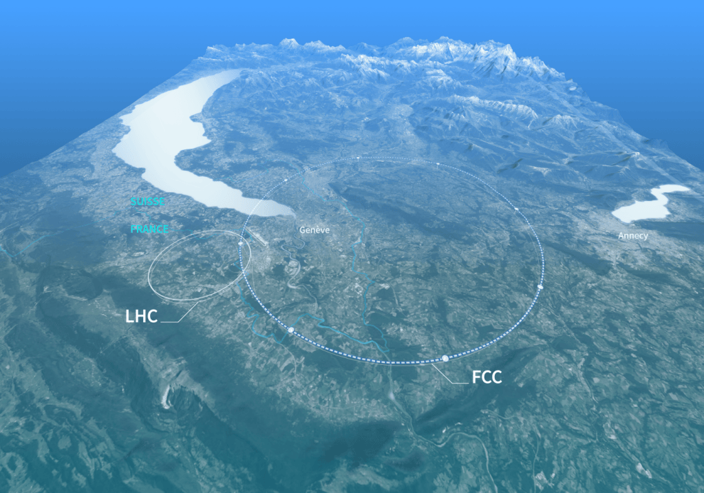
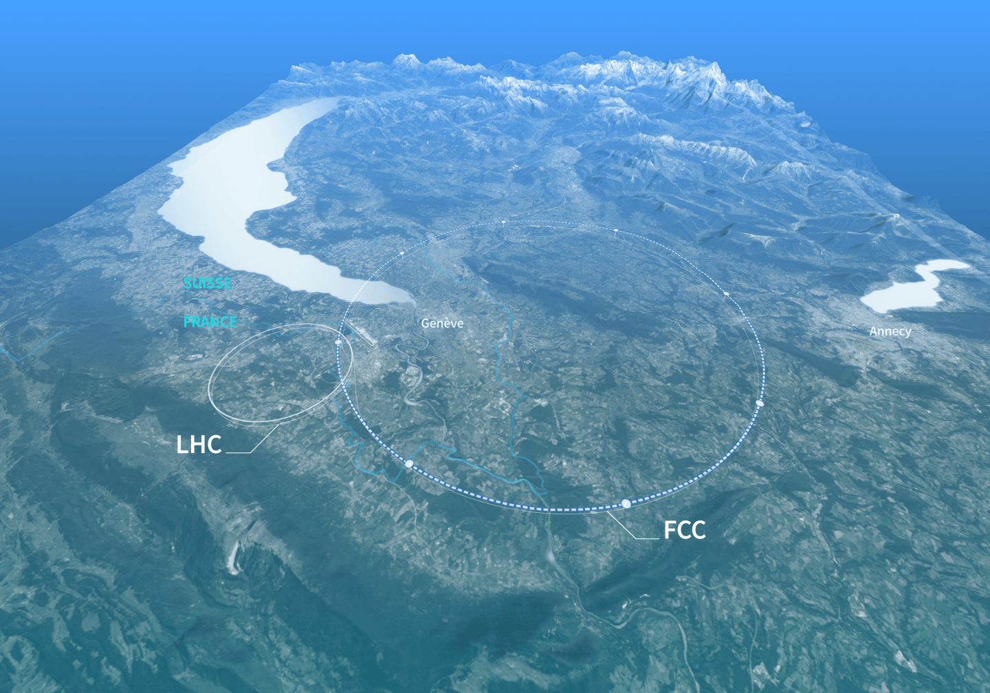
Figure 1. Schematic view of a proposed Future Circular Collider (FCC) location in the Geneva region, showing its ring alongside the existing LHC. Image credit: Daniel Dominguez/CERN, © 2025 CERN. Source: CERN Document Server, CERN-GRAPHICS-2025-002.
A quick reminder: what am I varying?
The reference distributions in this study came from Standard Model simulation. They represented an assumed Standard Model world, rather than measurements from a real experiment.
Against that reference, I tested a prediction consisting of:
Standard Model baseline + μ × an additional test contribution.
The parameter μ, pronounced “mu”, controls the size of the added component. At μ = 0, there is no extra contribution. At μ = 1, I add the nominal template once.
The templates were themselves derived from Standard Model simulation. This let me test the interpretation machinery with controlled inputs, without relying on the unresolved EFT event-generation workflow.
Using the Spey statistical backend, I scanned μ to examine where the fit was best and how it changed as the added contribution grew.
First: does the 13 TeV test behave sensibly?
The 13 TeV study used the fat-jet mass distribution as a closure test.
A closure test asks whether a procedure gives the expected behaviour in a controlled situation. Here, the reference and baseline were both SM-like, so the reference should not require an additional contribution.
The scan’s best-fit μ was effectively zero.
That was reassuring. My synthetic Standard Model reference was happy with the Standard Model baseline. A modest ambition, perhaps, but a useful place to start.
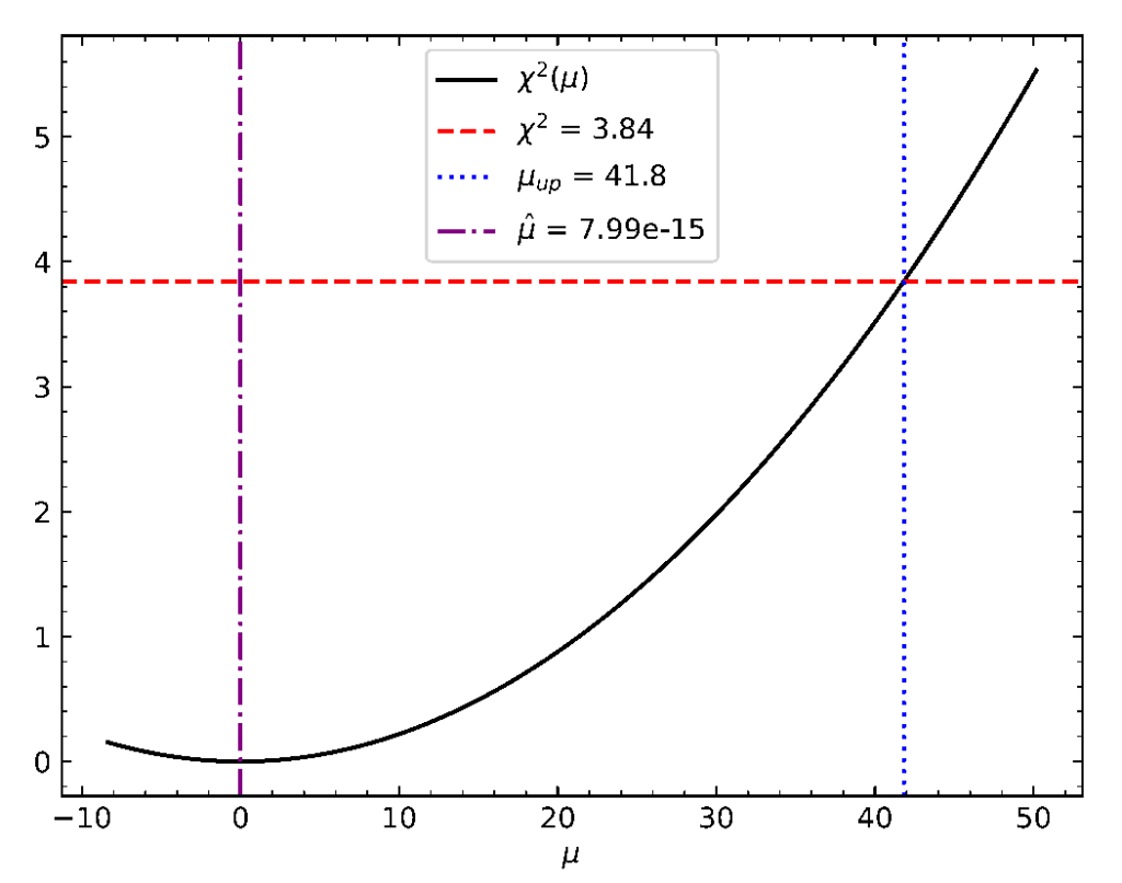
Figure 2. The 13 TeV scan. The black curve reaches its minimum near μ = 0. The blue vertical line marks the crossing of the red reference threshold at μ ≈ 41.8. Source: my UCL BSc project report.
The curve rises as the added contribution becomes larger. In this implementation, it reached the chosen threshold at μ ≈ 41.8—about 42 times the nominal added template.
That crossing was far above μ = 1. The nominal contribution therefore did not reach the threshold used in this scan.
The main achievement here was the expected qualitative behaviour of the connected workflow. The uncertainty treatment still needed checking before the crossing could receive a reliable confidence-level interpretation.
Then: the 85 TeV FCC-like study
For the 85 TeV setup, I examined the groomed mass of b-tagged Higgs-candidate fat jets.
Importantly, this distribution was taken before applying the explicit Higgs mass window. A peak near the Higgs mass could therefore tell me something useful about the reconstruction, rather than simply reflecting a requirement that I had already imposed.
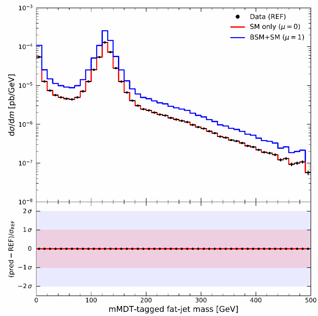
Figure 3. The 85 TeV candidate-mass distribution before the Higgs mass-window selection. Black markers are simulated pseudo-data; red is the SM baseline; blue includes the nominal added template. The original legend labels the blue curve “BSM+SM”, although this test used an SM-derived template. Source: my UCL BSc project report.
There was a clear feature around 125 GeV, consistent with the Higgs-candidate mass expected from the tagging procedure.
The reference and baseline agreed closely, while the added contribution raised the prediction around the peak and across the higher-mass region.
So the observable responded to an additional contribution in a physically relevant part of the distribution. The next question was how that response appeared in the statistical scan.
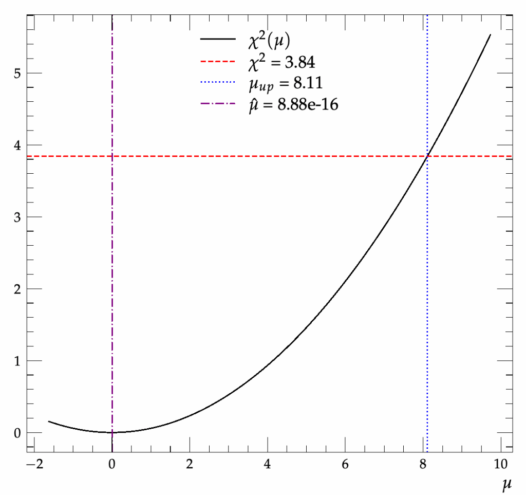
Figure 4. The 85 TeV scan. The minimum again lies near μ = 0, with the plotted threshold crossing at μ ≈ 8.11. Source: my UCL BSc project report.
Again, the best fit was effectively zero. The scan reached its threshold at μ ≈ 8.11, corresponding to about eight nominal templates.
The nominal μ = 1 contribution remained below that crossing.
Does 8.11 versus 41.8 prove an FCC improvement?
It is tempting to divide the two numbers and announce a dramatic improvement.
I would also quite like the arithmetic to finish the physics for me.
However, these were different benchmark setups using different observables. The meaning of one unit of μ also depends on how the added template is normalised.
The two crossings therefore do not isolate the effect of changing the collision energy.
Within its particular setup, the 85 TeV study showed a response to the added contribution and a lower crossing in template units. A controlled comparison of collider sensitivity would require consistent assumptions about observables, template definitions, luminosity, and uncertainties.
The unfinished part: uncertainties
This was the main limitation of the interpretation.
The simulated reference had very small uncertainties in some bins. In the 13 TeV distribution, even a modest difference between curves could consequently produce a large deviation when expressed in units of those uncertainties.
I also had not fully established how the Monte Carlo statistical uncertainty of the added template entered the calculation. Correlations between bins remained another unresolved issue.
These details matter. Shared uncertainties can make several bins move together, affecting how much independent information the distribution contains.
The lower panels of the comparison plots therefore needed caution. In particular, a reassuring-looking panel does not establish that every contribution’s uncertainty has been propagated correctly.
The scans also used the threshold value 3.84 shown by the red lines. Establishing the appropriate confidence-level interpretation required further statistical checks; the existence of a crossing alone did not complete that work.
What did this stage achieve?
The custom analysis could now produce distributions, construct a simulated reference, and run through Contur/Spey to obtain statistical scans.
The 13 TeV test returned the expected best fit near zero. The 85 TeV study produced a Higgs-sensitive mass distribution and a scan that responded to the added template.
Those were useful results from a working pipeline.
The numerical crossings remained provisional, and turning them into reliable constraints required better control of uncertainties and correlations. A direct EFT interpretation would also need validated predictions connecting the Wilson coefficients to the tested distributions.
The computer had successfully returned numbers. The remaining work was understanding exactly what those numbers deserved to mean.
Next, I’ll bring the UCL project together: what I set out to do, what I completed, and what I would tackle first if I continued it.

