
First, sorry for the delay. I was busy and lazy at the same time : (
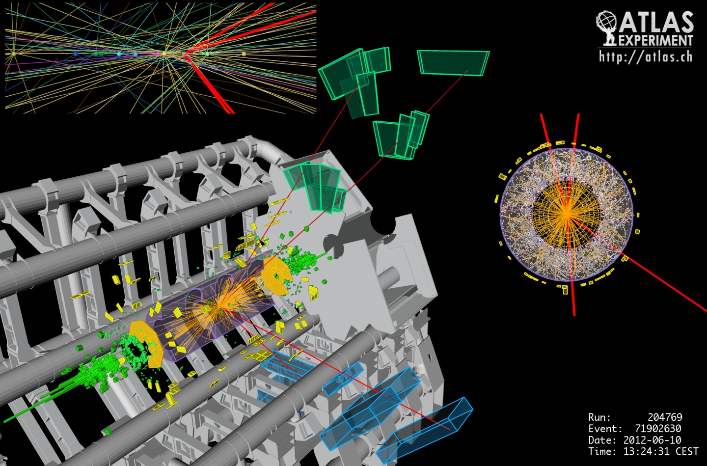
But here is a cool figure from ATLAS to get us started.
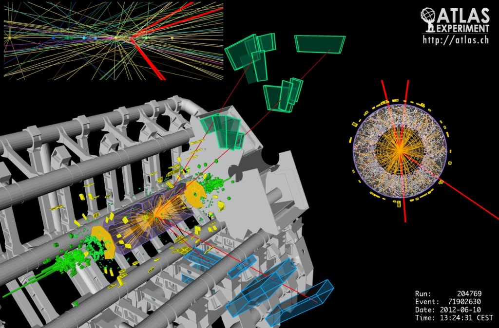
Figure 1. ATLAS event display of a candidate Higgs decay into four muons, H → ZZ* → 4μ, recorded on 10 June 2012. Image credit: ATLAS Collaboration, © 2012 CERN. Reproduced without modification under CC BY-SA 4.0. Original source: CERN Document Server.
Last time, I explained how my Rivet routine looks for boosted Higgs bosons: find a large jet, check its b-hadron content, examine its internal structure, and require a mass near the Higgs mass.
Getting that routine to produce tagged candidates was a useful milestone. The next question was harder: how many of those candidates would actually be Higgs bosons?
A background jet does not politely remove itself just because I have written a Higgs analysis.
My project studies a different decay channel from the ATLAS image above. I am looking at proton–proton collisions producing a Z boson and a Higgs boson together: pp → ZH. The Z decays into neutrinos, while the Higgs decays into a bottom quark and an antibottom quark.
At high transverse momentum, the two bottom quarks can end up inside one large jet. The neutrinos escape, leaving missing transverse momentum, or MET.
One lesson from the optimisation was that the generated sample has to match this target carefully. Changing jet settings cannot compensate for generating lots of events outside the final state I want.
I therefore focused the signal generation on Z bosons with transverse momentum above 400 GeV and explicitly selected invisible Z decays. This matters when quoting efficiencies: an efficiency measured in that restricted sample is conditional on those generation choices. It is not the fraction of all produced ZH events that an experiment would detect.
Within that sample, I varied three main settings: the MET requirement, the large-jet radius, and the grooming parameter z_cut.
A representative working point used MET above 400 GeV, a jet radius of 1.0, and z_cut = 0.1. It retained 217,297 tagged candidates from one million generated signal events—about 21.7%.
That was a useful working point, although a wider study would be needed to establish an optimum.
Then came the background.
The main process studied was Z production alongside a bottom quark and an antibottom quark, again with the Z decaying invisibly. It can produce the same broad ingredients as the signal: missing momentum and bottom-quark jets, without a Higgs decay providing the bottom-quark pair.
Stephen generated the background sample, and I brought the signal and background through the analysis for comparison, using one million simulated events of each.
Equal simulated sample sizes do not mean equal expected event rates. Those depend on the process cross sections, the assumed integrated luminosity, and the fraction surviving the selection:
Expected event count = cross section × integrated luminosity × selection efficiency.
This let me compare the expected surviving signal, S, with the expected surviving background, B.
I examined both S/B, the signal-to-background ratio, and S/√B—S divided by the square root of B—a simple approximation to statistical sensitivity.
They answer different questions. A selection can produce a cleaner sample while throwing away enough signal to make the measurement less sensitive.
The MET comparisons showed that trade-off. More demanding selections could suppress background, but they also reduced the signal yield. At the highest MET values, surviving simulated events became scarce, so apparently impressive ratios needed caution: large fluctuations in a nearly empty bin are not evidence of excellent tagging.
The result was a working procedure for studying signal and background together. It also remained a particle-level study, with detector effects and a fuller uncertainty treatment still ahead.
Meanwhile, difficulties establishing a reliable HEL-to-SMEFT event-generation workflow changed the direction of the project. The early EFT benchmarks remained useful exploratory studies, while the main analysis developed around a controlled Standard Model baseline.
That led to the next question: once I have these distributions, how do I turn them into a statement about an additional contribution?
For that, I needed to return to Contur—and work out how to construct a measurement for a collider that has not run yet.

